Understanding the bias-variance trade-off !

The bias-variance trade-off, remember? Models perform well for an "intermediate level of adaptability," according to the statement. In this blog, we will explore a different perspective of what the bias-variance trade-off means in terms of model training.
Introduction :
Recently, there has been a lot of discussion around the bias-variance trade-off (BVT). While the idea of BVT is simple, it can be difficult to understand. The BVT tradeoff states that while reducing the variance of a dataset will improve its predictive accuracy, it will also reduce its bias. So for example, if you have a dataset with 5 years worth of sales data, and you reduce the standard deviation from 50 to 20, you would reduce the average sale value from $100 to $80 but would also decrease the predicted number of sales from 500 to 300.
This graph gives a nice visual depiction of the trade-off that occurs when the bias-variance trade-off is at play. As we can see, increasing the variance improves the accuracy of the model, but this comes at the expense of reducing its bias. Essentially, the goal of a model should be to maximize its predictive accuracy while minimizing its bias. The trade-off occurs because minimizing bias means making less accurate predictions whereas maximizing accuracy means making less biased predictions.
When a dataset has a high variance, it means that many data points are far away from the mean and the possible ranges of these data points are extremely large. Since the range of possible values for a data point is proportional to its standard deviation, this means that the model will have to extrapolate beyond the available data to predict future values. Reducing the variance, however, reduces the number of data points that can be used to make predictions and increases the chance that a prediction will be wrong. These two factors cancel each other out to some extent and create a sort of "trade-off" between bias and variance.
This is why it is usually recommended that you build a model with a relatively high variance to account for outliers. However, you should keep this model flexible so that it can easily be adjusted to accommodate new data points as you collect them.
A trade-off perspective :
Bias-Variance is frequently referred to as a trade-off. When we talk about trade-offs, we often mean scenarios with two (or more) conflicting quantities where enhancing one weakens the other and vice versa. The exploration-exploitation trade-off in reinforcement learning is a well-known example, where increasing the exploration component (for instance, being -greedy) results in the agent exploiting the already-estimated high-value states less.
However, bias-variance is more of a decomposition. The decomposition of the expected test error (mean squared error) of a regression model into the three components of variance, bias, and irreducible error (caused by noise and internal variability) is demonstrated.
$$E(Loss) = Bias + Variance + Irreducible Error$$
Bias and variance, on the other hand, are not simple levers that you can pull to alter the error, unlike the exploration-exploitation trade-off where you can directly manipulate the 2 competing numbers. The test mistake is simply written in a different form, and bias and variance result from this decomposition.
Then why is it referred to as a trade-off? While more rigid models typically have high bias and low variance, flexible models typically have low bias and high variance. By controlling the regularisation, several parameters, and other aspects of the model, you can indirectly alter the bias and variance.
So, what's the catch?
When it comes to machine learning models, it’s also about finding the happy medium.
A model that is far too simplistic may result in significant bias and low variance. If a model contains too many parameters, it may result in high variance and low bias. As a result, our goal here is to locate the ideal position where neither overfitting nor underfitting occurs.
A low-variance model is typically less complicated and has a basic structure; nonetheless, it is subject to significant bias. Examples include Naive Bayes, Regression, and others. As a result, the model under fits since it is unable to recognize the signals in the data and hence cannot generate predictions on unseen data.
A low-bias model is typically more complicated and has a more flexible structure, but it is subject to large volatility. Decision Trees, Nearest Neighbors, and other techniques are examples of this. When a model becomes too complicated, it overfits because the model memorizes the noise in the data rather than the signals.
Click on this link to learn more about how to prevent overfitting, signals, and noise.
This is when the Trade-off enters the picture. To reduce overall error, we must find a happy medium between Bias and Variance. Let's have a look at Total Error.
The Math behind it :
Let's start with a simple formula where what we are trying to predict is ‘Y’ and the other covariates are ‘X’. The relationship between the two can be defined as:
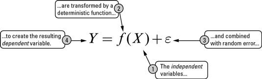
where the ‘e’ refers to the error term.
The expected squared error at a point x can then be defined as:
$$Err(x) = E[(Y-\hat{f}(x))^2]$$
which then produces :
$$Err(x) = (E[\hat{f}(x)]-f(x))^2 + E[(\hat{f}(x)-E[\hat{f}(x)])^2] + Irreducible Error$$
This can be defined better into :
$$Total Error = Bias^2 + Variance + Irreducible Error$$
Irreducible Error means the ‘noise’ that cannot be reduced in modeling - a way to reduce it would be through data cleaning.
Effect of Bias and Variance on the Total Error of your Model :
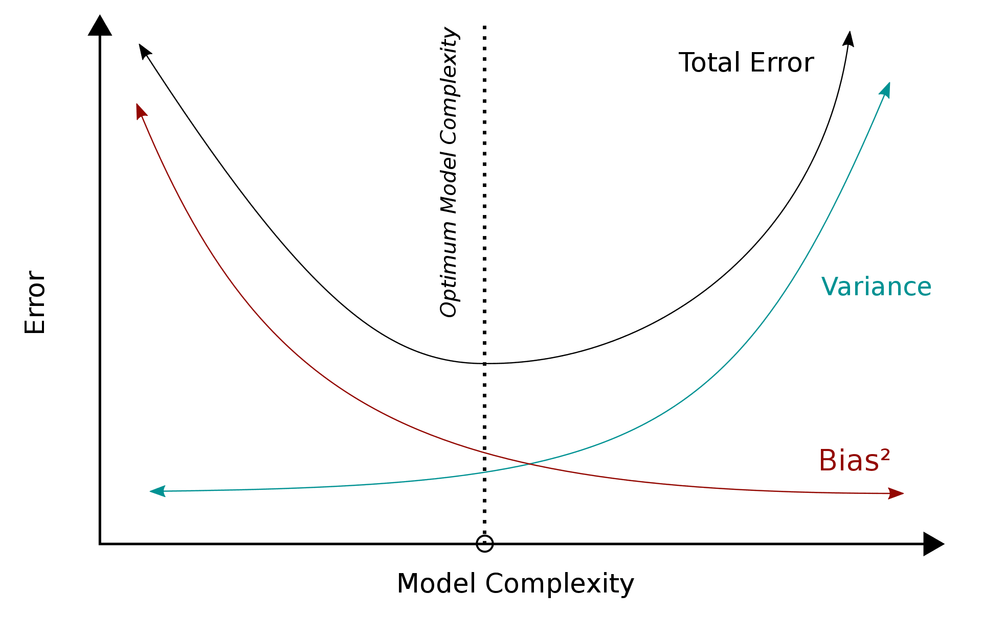
Figure I depicts the relationship between bias, variance, and total error. The x-axis shows our model's complexity, while the y-axis represents the error value.
Refer to Figure I :
We can observe that as the model's complexity rises, the bias decreases but the variance increases. This is because when the model grows in size, its potential to describe a function grows as well. If the model is large enough, it may memorize all of the training data, reducing the error to zero (if the Bayes error is zero). However, having an excessively complicated model will result in poor generalization despite high training performance. This is known as overfitting.
If your model is too simplistic, it will have a very high bias and a low variance. Even with training samples, the error would be quite large. If your model still performs poorly on training data after several epochs, this indicates that either your data contains corrupt labels or the model isn't complicated enough to mimic the underlying function. This is referred to as underfitting.
As seen in the graph, the total error decreases until it reaches the optimal complexity point. This is the point at which just the Bayes Error remains and the model performs optimally. At this moment, we have struck the correct balance between bias and variation.
Following are a few examples of what under-fitting, optimal-fitting and over-fitting looks like.

We see that the underlying noise is caught for models with a high variance (rightmost column). This results in excellent training performance but poor test performance. Because the generalization is the worst in this scenario. In contrast, models with a significant bias (leftmost column) are unable to reflect the underlying pattern in the data. As a result, the model performs badly even on training data. The optimum model is the best and most generalizable model because it contains the appropriate amount of bias and variation.
Putting Some Context :
Let's put some context (and graphs) here. Consider the below 1D dataset that was generated by the function ### and was perturbed by some Gaussian noise.
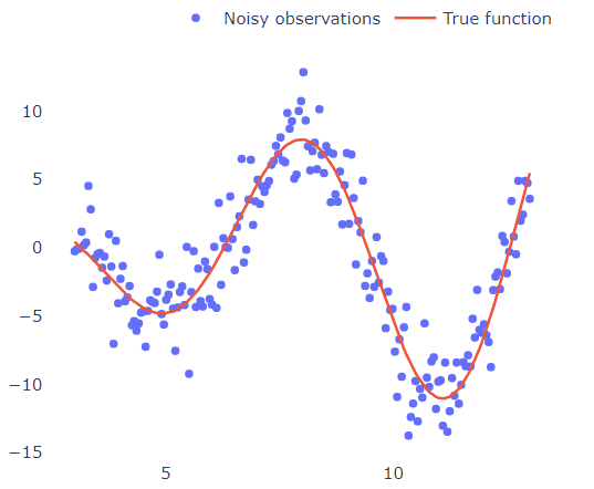
What if we wanted to fit a polynomial in these points?
We can look at the graph and, after taking a step back and straining our eyes pretty hard, draw a line that roughly crosses through all of the points (like the red line in the graph). We then see that for high and low x values, the y values tend to rise towards +infinity (if you squint hard enough), indicating that it should be an even-degree polynomial. The points then cut the x-axis four times (4 real roots), indicating that it must be a polynomial of at least four degrees. Finally, we see that the graph includes three turning points (from growing to decreasing or vice versa), suggesting that we have a 4-degree polynomial.
By "squinting our eyes," we essentially performed noise smoothing to view the "larger picture" rather than the minute and inconsequential fluctuations of the dataset. But how can we be certain that this is the best option?
Just throw a 1000-degree polynomial and see what happens
We could employ the most "complicated" model we can think to match the points because we can't be sure about the degree of a polynomial that would best mimic the underlying process, or we're just too bored to estimate it. We fit many polynomials of the increasing degree to see how they behave to validate this argument :
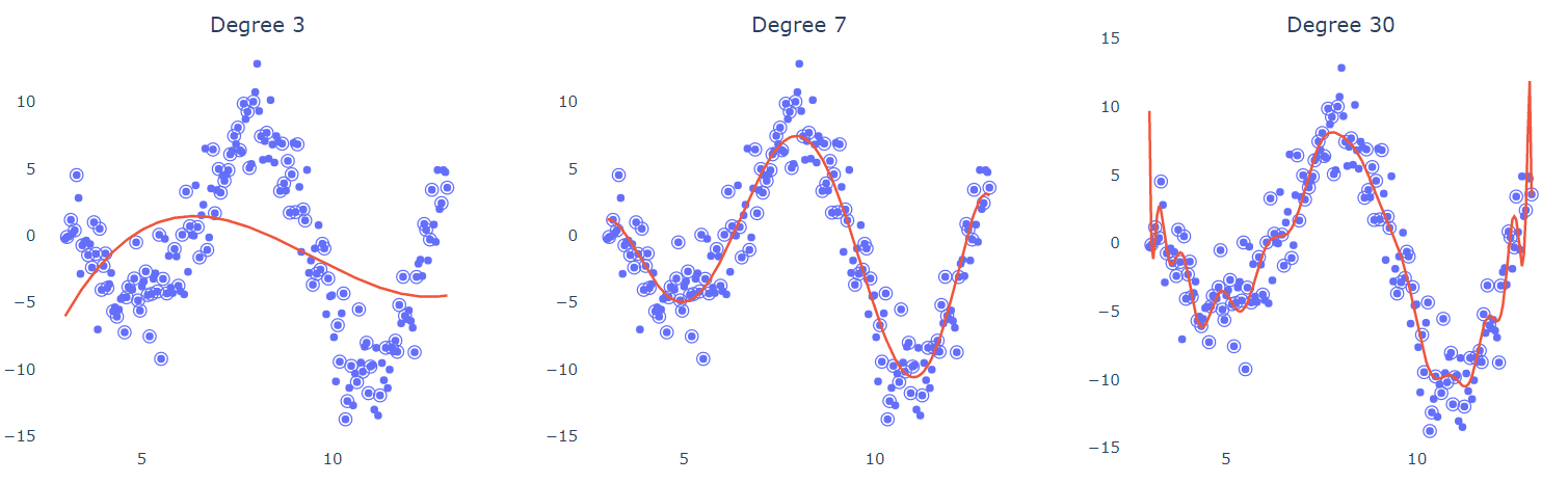
In each example, half of the points (circled) were used for training. The low-degree model (left) clearly cannot curl and bend sufficiently to suit the data. The 7-degree polynomial appears to travel between the spots gracefully as if it can disregard (smooth out) the noise. What's more intriguing is that the high-degree polynomial (right) attempts and succeeds in interpolating through the points. But is this what we want? What if you were given a different set of training points? Would the regression curve's form and predictions change?
The same fitting was done for different subsets of the data below, and the resulting curves are compared for variability. The findings for the 7-degree polynomial appear to be quite consistent.
As long as the training set is evenly sampled from the input space, the model is resistant to changes in the training set.

Now the same diagram for the 30-degree polynomial:
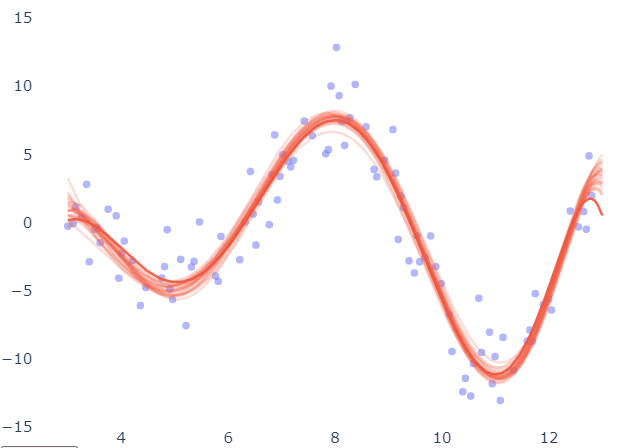
For different training sets, predictions appear to fluctuate up and down. The key implication is that we cannot trust such a model's forecast since, if we had a slightly different collection of data, the prediction of the same input sample would most likely alter.
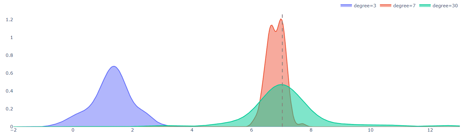
To demonstrate this point, the graphic below depicts the distributions of predictions for the three models when tested on a single test point (in this example, x=7) :
That's what Random Forests do :
The green distribution of the high-degree model in the accompanying graph demonstrates that predictions vary greatly among datasets. This is not a good model attribute since it is not resilient to tiny dataset changes. However, the average of the distribution is a far better predictor of the actual objective than the average value of the 7-degree model (red distribution). Averaging (bagging) the dataset over multiple realizations is a helpful approach that helps overcome overfitting and variation. This is exactly what Random Forests® accomplish, and they usually produce decent results without any adjusting.
Hopefully, these visuals will help explain how bias-variance affects model performance and why averaging many models may result in superior predictions.
Conclusion
If the blog has given you a better grasp of what Bias and Variance are and how they affect predictive modeling and you were able to understand the trade-off between the two and why it is critical to achieving that happy medium to develop the best-performing model that will not overfit or underfit - with a little math behind it, consider connecting with me in all my socials !


