Exploring the Depths of Transformers: A Deep Dive into the Inner Workings of NLP's Most Popular Model :

New deep-learning models are being launched at an increasing rate, and it can be difficult to keep up with all of the new developments. Yet, one neural network model, in particular, has shown to be very successful for common natural language processing tasks. The model is known as a Transformer, and it employs numerous ways and mechanisms, which I will discuss below. The publications I mention in the essay provide a more extensive and quantitative explanation.

Part 1: Sequence to Sequence Learning and Attention :

In the paper 'Attention Is All You Need,' transformers and a sequence-to-sequence architecture are discussed. Sequence-to-Sequence (Seq2Seq) is a neural network that converts one sequence of components into another, for as the sequence of words in a phrase. (Considering the name, this should come as no surprise.)

Seq2Seq models excel at translation, which involves transforming a series of words from one language into a sequence of other words in another. Long-Short-Term Memory (LSTM)-based models are a frequent choice for this sort of model. When dealing with sequence-dependent data, the LSTM modules may provide meaning to the sequence while remembering (or forgetting) the bits that are essential to them (or unimportant). Sentences, for example, are sequence-dependent because the order of the words is critical for comprehension. With this type of data, LSTM are an obvious choice.

An Encoder and a Decoder are used in Seq2Seq models. The Encoder converts the input sequence into a higher dimensional space (n-dimensional vector). The abstract vector is sent via the Decoder, which converts it into an output sequence. The output sequence might be in another language, symbols, a replica of the input, or something else entirely.

Consider the Encoder and Decoder to be human interpreters who can only communicate in two languages. Their first language is their mother tongue, which varies between them (for example, German and French), and their second language is a fictional one they share. The Encoder transforms the German statement into the other language it understands, namely the fictitious language, to translate it into French. Because the Decoder can read that imagined language, it can now convert it into French. The model (which consists of an Encoder and Decoder) can convert German into French!

Assume that neither the Encoder nor the Decoder is proficient in the imagined language at first. We train them (the model) on a large number of instances to learn it.

A single LSTM for each of the Seq2Seq model's Encoder and Decoder is a relatively simple choice.

You're wondering when the Transformer will make an appearance, aren't you?

We need one more technical detail to make Transformers easier to understand: Attention. The attention mechanism looks at an input sequence and decides at each step which other parts of the sequence are important. It sounds abstract, but let me clarify with an easy example: When reading this text, you always focus on the word you read but at the same time your mind still holds the important keywords of the text in memory to provide context.

For a given sequence, an attention mechanism operates similarly. Consider the human Encoder and Decoder in our example. Instead of just writing down the translation of the sentence in the imaginary language, imagine that the Encoder also writes down keywords that are important to the semantics of the sentence and gives them to the Decoder in addition to the regular translation. Because the Decoder understands which portions of the phrase are significant and which key elements provide context, the additional keywords make translation considerably easier.

In other words, for each input that the LSTM (Encoder) reads, the attention mechanism takes into account several other inputs at the same time and decides which ones are important by attributing different weights to those inputs. The Decoder will then take as input the encoded sentence and the weights provided by the attention mechanism. To learn more about attention, see this article. And for a more scientific approach than the one provided, read about different attention-based approaches for Sequence-to-Sequence models in this great paper called ‘Effective Approaches to Attention-based Neural Machine Translation’.

Part 2: The Transformer :

The paper 'Attention Is All You Need' presents the Transformer architecture. It employs the attention mechanism that we observed before, as the title suggests. Transformer, like LSTM, is an architecture for transforming one sequence into another using two components (Encoder and Decoder), however, it varies from the previously described/existing sequence-to-sequence models in that it does not employ Recurrent Networks (GRU, LSTM, etc.).

Recurrent Networks were, until now, one of the best ways to capture the timely dependencies in sequences. However, the team presenting the paper proved that architecture with only attention mechanisms without any RNN (Recurrent Neural Networks) can improve the results in translation tasks and other tasks! One improvement on Natural Language Tasks is presented by a team introducing BERT: BERT: Pre-training of Deep Bidirectional Transformers for Language Understanding.

So, precisely what is a Transformer? Because a picture is worth a thousand words, we'll start there!

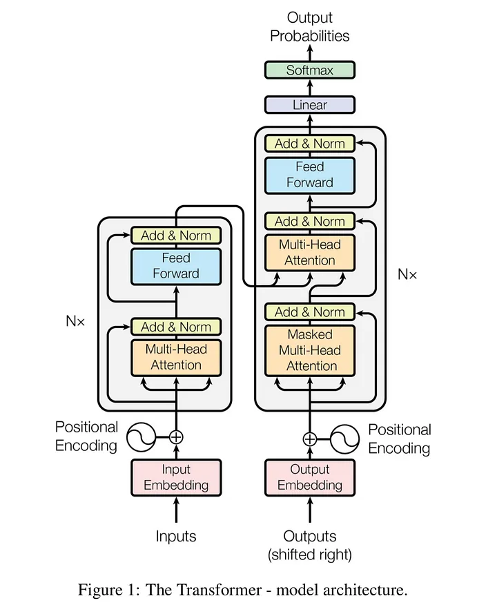
On the left is the Encoder, and on the right is the Decoder. Encoder and Decoder are both made up of modules that may be stacked on top of each other numerous times, as shown by Nx in the diagram. We can see that the modules are mostly made up of Multi-Head Attention and Feed Forward layers. Because we cannot utilise strings directly, the inputs and outputs (target phrases) are first embedded in an n-dimensional space.

The positional encoding of the various words is a minor but critical component of the model. We need to give every word/part in our sequence a relative location because a sequence depends on the order of its constituents and we don't have any recurrent networks that can recall how sequences are fed into a model. These places are added to each word's embedded representation (n-dimensional vector).

Let’s have a closer look at these Multi-Head Attention bricks in the model:

Let’s start with the left description of the attention-mechanism. It’s not very complicated and can be described by the following equation:

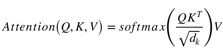
Q is a matrix containing the query (vector representation of one word in the sequence), K is all the keys (vector representations of all the words in the sequence), and V is the values (vector representations of all the words in the sequence). V is the same word sequence as Q for the encoder and decoder, multi-head attention modules. Nevertheless, for the attention module, which considers the encoder and decoder sequences, V differs from the sequence represented by Q.

To put it another way, the values in V are multiplied and summed with some attention-weights a, where our weights are specified as:

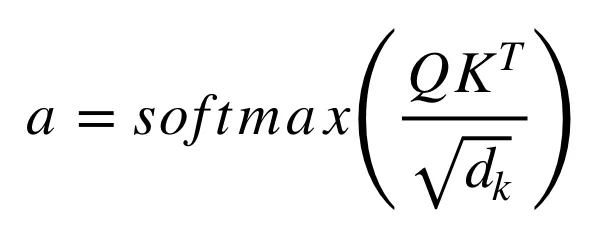
This means that the weights an are defined by how each word in the sequence (represented by Q) is impacted by the rest of the words in the sequence (represented by K). Moreover, the SoftMax function is applied to the weights a, resulting in a distribution between 0 and 1. These weights are then applied to all of the words introduced in V throughout the sequence (same vectors than Q for the encoder and decoder but different for the module that has encoder and decoder inputs).

The diagram on the right shows how this attention mechanism may be parallelized into many mechanisms that can be employed concurrently. The attention mechanism is repeated several times using Q, K, and V linear projections. This enables the system to learn from various representations of Q, K, and V, which benefits the model. These linear representations are created by multiplying Q, K, and V by weight matrices W learned during training.

These matrices Q, K, and V differ for each location of the attention modules in the structure, depending on whether they are in the encoder, decoder, or between the encoder and decoder. We wish to attend to either the entire encoder input sequence or a portion of the decoder input sequence. The multi-head attention module that connects the encoder and decoder will ensure that the encoder input sequence, together with the decoder input sequence, is taken into consideration up to a specific location.

A pointwise feed-forward layer follows the multi-attention heads in both the encoder and decoder. This little feed-forward network contains the same parameters for each position, which may be thought of as a distinct, identical linear transformation of each element in the provided sequence.

Training :

How do you train such a "beast"? Training and inferring on Seq2Seq models differ from traditional classification problems. The same may be said with Transformers.

We know that two phrases in separate languages that are translations of each other are required to train a model for translation tasks. We can begin training our model after we have a large number of phrase pairings. Assume we wish to translate from French to German. Our encoded input will be a French text, whereas the decoder's input will be a German sentence. The decoder input, on the other hand, will be moved to the right by one place. Why do you ask?

One reason is that we don't want our model to learn how to replicate our decoder input during training; instead, we want it to learn that given an encoder sequence and a certain decoder sequence that the model has already seen, we can predict the next word/character.

If the decoder sequence is not shifted, the model learns to simply 'copy' the decoder input, because the target word/character for the position I am the word/character I in the decoder input. As a result of moving the decoder input by one place, our model must predict the target word/character for the position I despite only seeing the words/characters 1,..., i-1 in the decoder sequence. This inhibits our model from learning how to copy and paste. Because the first slot of the decoder input would normally be empty due to the right shift, we fill it with a start-of-sentence token. Similarly, to identify the conclusion of the decoder input sequence, we insert an end-of-sentence token, which is likewise appended to the target output phrase. In a moment, we’ll see how that is useful for inferring the results.

This is true for Seq2Seq models and for the Transformer. In addition to the right-shifting, the Transformer applies a mask to the input in the first multi-head attention module to avoid seeing potential ‘future’ sequence elements. This is specific to the Transformer architecture because we do not have RNNs where we can input our sequence sequentially. Here, we input everything together and if there were no masks, the multi-head attention would consider the whole decoder input sequence at each position.

The process of feeding the correct shifted input into the decoder is also called Teacher-Forcing, as described in this blog.

The target sequence we want for our loss calculations is simply the decoder input (German sentence) without shifting it and with an end-of-sequence token at the end.

Inference

Inferring with those models is different from the training, which makes sense because in the end we want to translate a French sentence without having the German sentence. The trick here is to re-feed our model for each position of the output sequence until we come across an end-of-sentence token.

A more step-by-step method would be:

• Input the full encoder sequence (French sentence) and as decoder input, we take an empty sequence with only a start-of-sentence token on the first position. This will output a sequence where we will only take the first element.

• That element will be filled into the second position of our decoder input sequence, which now has a start-of-sentence token and a first word/character in it.

• Input both the encoder sequence and the new decoder sequence into the model. Take the second element of the output and put it into the decoder input sequence.

• Repeat this until you predict an end-of-sentence token, which marks the end of the translation. We see that we need multiple runs through our model to translate our sentence.

I hope that these descriptions have made the Transformer architecture a little bit clearer for everybody starting with Seq2Seq and encoder-decoder structures.

Part 3: Use-Case ‘Transformer for Time-Series’ :

We have seen the Transformer architecture and we know from literature and the ‘Attention is All you Need’ authors that the model does extremely well in language tasks. Let’s now test the Transformer in a use case.

Instead of a translation task, let’s implement a time-series forecast for the hourly flow of electrical power in Texas, provided by the Electric Reliability Council of Texas (ERCOT). You can find the hourly data here.

A great detailed explanation of the Transformer and its implementation is provided by harvardnlp. If you want to dig deeper into the architecture, I recommend going through that implementation.

Since we can use LSTM-based sequence-to-sequence models to make multi-step forecast predictions, let’s have a look at the Transformer and its power to make those predictions. However, we first need to make a few changes to the architecture since we are not working with sequences of words but with values. Additionally, we are doing an auto-regression and not a classification of words/characters.

The Data

The available data gives us an hourly load for the entire ERCOT control area. I used the data from the years 2003 to 2015 as a training set and the year 2016 as a test set. Having only the load value and the timestamp of the load, I expanded the timestamp to other features. From the timestamp, I extracted the weekday to which it corresponds and one-hot encoded it. Additionally, I used the year (2003, 2004, …, 2015) and the corresponding hour (1, 2, 3, …, 24) as the value itself. This gives me 11 features in total for each hour of the day. For convergence purposes, I also normalized the ERCOT load by dividing it by 1000.

To predict a given sequence, we need a sequence from the past. The size of those windows can vary from use-case to use-case but here in our example, I used the hourly data from the previous 24 hours to predict the next 12 hours. It helps that we can adjust the size of those windows depending on our needs. For example, we can change that to daily data instead of hourly data.

Changes to the model from the paper

As a first step, we need to remove the embeddings, since we already have numerical values in our input. An embedding usually maps a given integer into an n-dimensional space. Here instead of using the embedding, I simply used a linear transformation to transform the 11-dimensional data into an n-dimensional space. This is similar to the embedding with words.

We also need to remove the SoftMax layer from the output of the Transformer because our output nodes are not probabilities but real values.

After those minor changes, the training can begin!

As mentioned, I used teacher forcing for the training. This means that the encoder gets a window of 24 data points as input and the decoder input is a window of 12 data points where the first one is a ‘start-of-sequence’ value and the following data points are simply the target sequence. Having introduced a ‘start-of-sequence’ value at the beginning, I shifted the decoder input by one position with regard to the target sequence.

I used an 11-dimensional vector with only -1’s as the ‘start-of-sequence’ values. Of course, this can be changed and perhaps it would be beneficial to use other values depending on the use case but for this example, it works since we never have negative values in either dimension of the input/output sequences.

The loss function for this example is simply the mean squared error.

Results

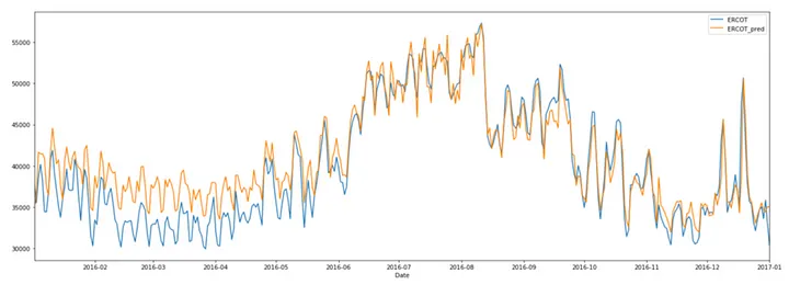
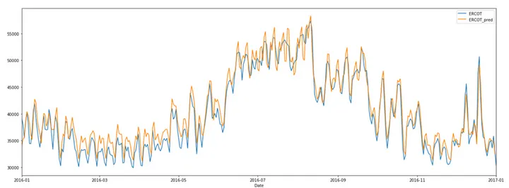
The two plots below show the results. I took the mean value of the hourly values per day and compared it to the correct values. The first plot shows the 12-hour predictions given the 24 previous hours. For the second plot, we predicted one hour given the 24 previous hours. We see that the model can catch some fluctuations very well. The root means squared error for the training set is 859 and for the validation set, it is 4,106 for the 12-hour predictions and 2,583 for the 1-hour predictions. This corresponds to a mean absolute percentage error of the model prediction of 8.4% for the first plot and 5.1% for the second one.

Summary

The results suggest that the Transformer design may be used for time-series forecasting. Yet, the examination reveals that the more steps we wish to anticipate, the greater the mistake. The first graph (Figure 3) was created by predicting the future 12 hours using the previous 24 hours. If we merely anticipate one hour, the results are substantially better, as seen in the second graph (Figure 4).

There's lots of flexibility to experiment with the Transformer's settings, such as the number of decoder and encoder layers, etc. This was not intended to be a flawless model, and the results would most likely improve with more tuning and training.

Thank you for reading, and I hope I was able to clear up some misconceptions for those who are just getting started with Deep Learning!